The intent of this blog is to summarize and document a personal project I did after completion of a “specialization” on Machine Learning on Coursera platform. This blog documents application of Bernoulli Mixture Models to unsupervised learning of handwritten digits dataset.
Reference/Inspiration: Pattern Recognition and Machine Learning by Christopher M. Bishop. Chapter 9, Figure 9.10.
Dataset: MNIST Handwritten Digits.
Model: Bernoulli Mixture Models
Algorithm: Expectation-Maxization
Mixture of Bernoulli Distribution
First, consider a single multivariate random variable \(\mathbf{x}\) with Bernoulli distribution of \(D\) independent binary variables \(x_i \in \{0, 1\}\), where \(i = 1,...,D\), each of which is in turn a univariate Bernoulli distribtion with parameter \(\mu_i\),
\[p(\mathbf{x}\,|\, \boldsymbol{\mu}) = \displaystyle\prod_{i=1}^D \mu_i^{x_i}(1-\mu_i)^{(1-x_i)}\]where, \(\mathbf{x} = (x_1,...,x_D)^T\), and \(\boldsymbol{\mu} = (\mu_1,...,\mu_D)^T\).
Now consider a finite mixture of \(K\) multivariate Bernoulli distributions given by,
\(p(\mathbf{x}\,|\, \boldsymbol{\mu}, \boldsymbol{\pi}) = \displaystyle\sum_{k=1}^K \pi_k p(\mathbf{x}\,|\,\boldsymbol{\mu}_k)\)
where,
\(\boldsymbol\mu = \{\boldsymbol\mu_1,...,\boldsymbol\mu_K\}\)
or
\(\mu_{ki} =
\begin{pmatrix}
\mu_{11} & \mu_{12} & \cdots & \mu_{1D} \\
\mu_{2,1} & \mu_{22} & \cdots & \mu_{2D} \\
\vdots & \vdots & \ddots & \vdots \\
\mu_{K1} & \mu_{K2} & \cdots & \mu_{KD}
\end{pmatrix}\),
\(\boldsymbol\pi = \{\pi_1,...,\pi_K\}\), and
Given a data set of \(\mathbf{X} = \left\{\mathbf{x}_1,...,\mathbf{x}_N\right\}\), with each observation represented as a mixture of K Bernoulli distributions, then the log likelihood function is:
\[\mathrm{ln}\,p(\mathbf{X}\,|\,\boldsymbol{\mu},\boldsymbol{\pi}) = \displaystyle\sum_{n=1}^N\mathrm{ln}\left\{\displaystyle\sum_{k=1}^K \pi_{k}\,p(\mathbf{x}_n\,|\,\boldsymbol{\mu}_k)\right\}\]The appearance of the summation inside the logarithm in the above function means maximixum likelihood solution no longer has a closed form solution.
To maximize the log likelihood function using Expection-Maximization approach, consider an explicit latent variable \(\mathbf{z}\) associated with each observation \(\mathbf{x}\), where \(\mathbf{z}=(z_1,...,z_K)^T\) is a binary K-dimensional variable having a single component equal to 1, and all others set to 0. The latent variable \(\mathbf{z}\) can be considered as a membership indicator for each observation. The marginal distribution of \(\mathbf{z}\) is specified in terms of the mixing coefficients \(\pi_k\), such that \(p(z_k = 1) =\,\pi_k\), or \(p(\mathbf{z}\,|\,\boldsymbol{\pi}) = \displaystyle\prod_{k=1}^K \pi_k^{z_k}\) We can write the conditional distribution of \(\mathbf{x}\), given the latent variable as \(p(\mathbf{x}\,|\,\mathbf{z},\boldsymbol{\mu}) = \displaystyle\prod_{k=1}^K\,p(\mathbf{x}\,|\,\boldsymbol{\mu}_k)^{z_k}\)
Now formulate the probability of the complete-data (observed \(\mathbf{x}\) and latent \(\mathbf{z}\)) using Bayes’ theorem, \(p(\mathbf{x},\mathbf{z}) = p(\mathbf{x}\,|\,\mathbf{z})p(\mathbf{z})\). For the complete-data, the probability is
\[\begin{align*} p(\mathbf{X},\mathbf{Z}\,|\,\boldsymbol{\mu},\boldsymbol{\pi}) &= \displaystyle\prod_{n=1}^{N}\,p(\mathbf{x}\,|\,\mathbf{z},\boldsymbol{\mu})\,p(\mathbf{z}\,|\,\boldsymbol{\pi}) \\ &=\displaystyle\prod_{n=1}^{N}\,\displaystyle\prod_{k=1}^{K} \pi_{k}^{z_{nk}} \left( p(\mathbf{x}\,|\,\mu_{k}\right)^{z_{nk}} \\ & = \displaystyle\prod_{n=1}^{N}\,\displaystyle\prod_{k=1}^{K} \pi_{k}^{z_{nk}} \left( \displaystyle\prod_{i=1}^D \mu_{ki}^{x_{ni}}(1-\mu_{ki})^{(1-x_{ni})}\right)^{z_{nk}} \\ \end{align*}\]The corresponding complete-data log likelihood functions is:
\[\begin{align*} \mathrm{ln}\,p(\mathbf{X},\mathbf{Z}\,|\,\boldsymbol{\mu},\boldsymbol{\pi}) &= \displaystyle\sum_{n=1}^{N}\,\displaystyle\sum_{k=1}^{K} z_{nk} \left\{ \mathrm{ln}\,\left(\pi_{k}\,\displaystyle\prod_{i=1}^D \mu_{ki}^{x_{ni}}(1-\mu_{ki})^{(1-x_{ni})}\right)\right\}\\ &=\displaystyle\sum_{n=1}^{N}\,\displaystyle\sum_{k=1}^{K} z_{nk} \left\{\mathrm{ln}\,\pi_{k}+ \displaystyle\sum_{i=1}^D \mathrm{ln}\,\left(\mu_{ki}^{x_{ni}}(1-\mu_{ki})^{(1-x_{ni})}\right)\right\}\\ &=\displaystyle\sum_{n=1}^{N}\,\displaystyle\sum_{k=1}^{K} z_{nk} \left\{\mathrm{ln}\,\pi_{k}+ \displaystyle\sum_{i=1}^D \left[x_{ni}\,\mathrm{ln}\,\mu_{ki}+(1-x_{ni})\,\mathrm{ln}\,(1-\mu_{ki})\right]\right\}\\ \end{align*}\]Notice that the above log likelihood function can be considered as a linear combination of \(z_{nk}\). Since the expectation of a sum is the sum of the expectations, we can write the expectation of the complete-data log likelihood functions with respect to the posterior distribution of the latent variable as:
\[\mathbb{E}_{\mathbf{Z}}\left[\mathrm{ln}\,p(\mathbf{X},\mathbf{Z}\,|\,\boldsymbol{\mu},\boldsymbol{\pi})\right] = \displaystyle\sum_{n=1}^{N}\,\displaystyle\sum_{k=1}^{K} \gamma(z_{nk}) \left\{\mathrm{ln}\,\pi_{k}+ \displaystyle\sum_{i=1}^D \left[x_{ni}\,\mathrm{ln}\,\mu_{ki}+(1-x_{ni})\,\mathrm{ln}\,(1-\mu_{ki})\right]\right\}\]where, \(\gamma(z_{nk}) = \mathbb{E}[z_{nk}]\) is the posterior probability or responsibility of the mixture component \(k\) given the data point \(x_n\).
E-M Algorithm for the Mixture of Bernoulli Distributions:
With the above background, the E-M algorithm takes the following form.
E-Step:
Calculation of the responsibilites make the E step of the E-M algorithm.
M-Step:
Maximizing the expectation of the complete-data log likelihood with respect to \(\boldsymbol\mu_k\) and \(\boldsymbol\pi_k\) yields the M step of the E-M algorithm:
and
\[\pi_{k}\,=\,\frac{N_k}{N}\]where, \(N_k\,=\,\displaystyle\sum_{n=1}^N\,\gamma(z_{nk})\)
import numpy as np
import matplotlib.pyplot as plt
%matplotlib inline

from sklearn.datasets import fetch_mldata

mnist = fetch_mldata("MNIST original")
mnist.data.shape
'''
MNIST data is in grey scale [0, 255].
Convert it to a binary scale using a threshold of 128.
'''
mnist3 = (mnist.data/128).astype('int')
def show(image):
    '''
    Function to plot the MNIST data
    '''
    fig = plt.figure()
    ax = fig.add_subplot(1,1,1)
    imgplot = ax.imshow(image, cmap=plt.cm.Greys)
    imgplot.set_interpolation('nearest')
    ax.xaxis.set_ticks_position('top')
    ax.yaxis.set_ticks_position('left')
    plt.show()
def bernoulli(data, means):
    '''To compute the probability of x for each bernouli distribution
    data = N X D matrix
    means = K X D matrix
    prob (result) = N X K matrix
    '''
    N = len(data)
    K = len(means)
    #compute prob(x/mean)
    # prob[i, k] for ith data point, and kth cluster/mixture distribution
    prob = np.zeros((N, K))

    for i in range(N):
        for k in range(K):
            prob[i,k] = np.prod((means[k]**data[i])*((1-means[k])**(1-data[i])))

    return prob
def respBernoulli(data, weights, means):
    '''To compute responsibilities, or posterior probability p(z/x)
    data = N X D matrix
    weights = K dimensional vector
    means = K X D matrix
    prob or resp (result) = N X K matrix
    '''
    #step 1
    # calculate the p(x/means)
    prob = bernoulli(data, means)

    #step 2
    # calculate the numerator of the resp.s
    prob = prob*weights

    #step 3
    # calcualte the denominator of the resp.s
    row_sums = prob.sum(axis=1)[:, np.newaxis]

    # step 4
    # calculate the resp.s
    try:
        prob = prob/row_sums
        return prob
    except ZeroDivisionError:
        print("Division by zero occured in reponsibility calculations!")
def bernoulliMStep(data, resp):
    '''Re-estimate the parameters using the current responsibilities
    data = N X D matrix
    resp = N X K matrix
    return revised weights (K vector) and means (K X D matrix)
    '''
    N = len(data)
    D = len(data[0])
    K = len(resp[0])

    Nk = np.sum(resp, axis=0)
    mus = np.empty((K,D))

    for k in range(K):
            mus[k] = np.sum(resp[:,k][:,np.newaxis]*data,axis=0) #sum is over N data points
            try:
                mus[k] = mus[k]/Nk[k]
            except ZeroDivisionError:
                print("Division by zero occured in Mixture of Bernoulli Dist M-Step!")
                break

    return (Nk/N, mus)
def llBernoulli(data, weights, means):
    '''To compute expectation of the loglikelihood of Mixture of Beroullie distributions
    Since computing E(LL) requires computing responsibilities, this function does a double-duty
    to return responsibilities too
    '''
    N = len(data)
    K = len(means)

    resp = respBernoulli(data, weights, means)

    ll = 0
    for i in range(N):
        sumK = 0
        for k in range(K):
            try:
                temp1 = ((means[k]**data[i])*((1-means[k])**(1-data[i])))
                temp1 = np.log(temp1.clip(min=1e-50))

            except:
                print("Problem computing log(probability)")
            sumK += resp[i, k]*(np.log(weights[k])+np.sum(temp1))
        ll += sumK

    return (ll, resp)
def mixOfBernoulliEM(data, init_weights, init_means, maxiters=1000, relgap=1e-4, verbose=False):
    '''EM algo fo Mixture of Bernoulli Distributions'''
    N = len(data)
    D = len(data[0])
    K = len(init_means)

    #initalize
    weights = init_weights[:]
    means = init_means[:]
    ll, resp = llBernoulli(data, weights, means)
    ll_old = ll

    for i in range(maxiters):
        if verbose and (i % 5 ==0):
            print("iteration {}:".format(i))
            print("   {}:".format(weights))
            print("   {:.6}".format(ll))

        #E Step: calculate resps
        #Skip, rolled into log likelihood calc
        #For 0th step, done as part of initialization

        #M Step
        weights, means = bernoulliMStep(data, resp)

        #convergence check
        ll, resp = llBernoulli(data, weights, means)
        if np.abs(ll-ll_old)<relgap:
            print("Relative gap:{:.8} at iternations {}".format(ll-ll_old, i))
            break
        else:
            ll_old = ll

    return (weights, means)
from sklearn.utils import shuffle

def pickData(digits, N):
    sData, sTarget = shuffle(mnist3, mnist.target, random_state=30)
    returnData = np.array([sData[i] for i in range(len(sData)) if sTarget[i] in digits])
    return shuffle(returnData, n_samples=N, random_state=30)

def experiments(digits, K, N, iters=50):
    '''
    Picks N random points of the selected 'digits' from MNIST data set and
    fits a model using Mixture of Bernoulli distributions.
    And returns the weights and means.
    '''

    expData = pickData(digits, N)

    D = len(expData[0])

    initWts = np.random.uniform(.25,.75,K)
    tot = np.sum(initWts)
    initWts = initWts/tot

    #initMeans = np.random.rand(10,D)
    initMeans = np.full((K, D), 1.0/K)

    return mixOfBernoulliEM(expData, initWts, initMeans, maxiters=iters, relgap=1e-15)
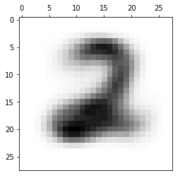
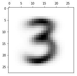
finWeights, finMeans = experiments([2,3,9], 3, 1000)
[show(finMeans[i].reshape(28,28)) for i in range(len(finMeans))]
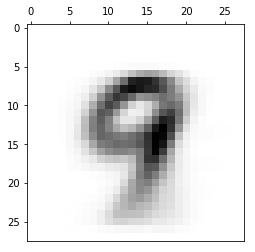
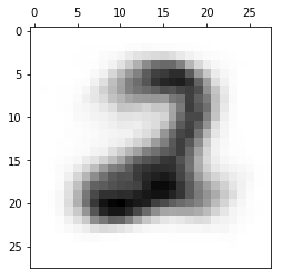
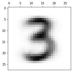
[None, None, None]
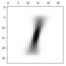
finWeights, finMeans = experiments([1,2,3,7], 4, 5000)
[show(finMeans[i].reshape(28,28)) for i in range(len(finMeans))]
print(finWeights)

[ 0.26757071 0.24729179 0.23207817 0.25305934]
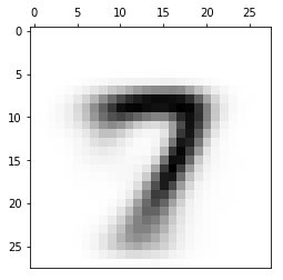
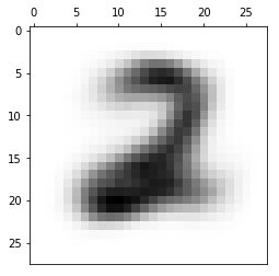
finWeights, finMeans = experiments([2,3,7], 4, 3000)
[show(finMeans[i].reshape(28,28)) for i in range(len(finMeans))]
print(finWeights)
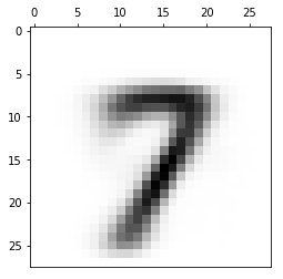
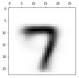
[ 0.1912005 0.15238828 0.34022079 0.31619044]