Introduction
Central banks across the world maintain gold reserves to guarantee the money of their depositors, foreign-debt creditors, and currency holders. Central banks also use gold reserves as a means to control inflation and strengthen their country’s financial standing. In addition, gold is used by finance companies, global institutions, money managers and individual investors to hedge against inflation and to diversify their portfolios. As a precious metal, gold is popular for jewelry and ornamentation.
Given the standing of gold’s popularity in the contemporary world, forecasting its price is a widely explored topic and interesting to multiple global institutions and small & large scale investors. It is also a complex problem given gold’s price fluctuations are not entirely based on supply and demand, but also depends on a multitude of geo-political and financial factors.
Methodology
The approach used for this analysis has three steps: data collection/assembly step, model building step, and an evaluation step.

Data Collection and Assembly
The independent variables considered for this analysis include economic and market factors like S&P 500, Dow Jones Industrial average, FTSE 100 Index, treasury bond rates, bank interest rates, US Dollar Index; and other commodity indicators like silver, platinum, palladium and crude oil prices. In addition, Gold Futures were also considered to reflect market expectation of future gold prices. A number of studies reviewed as part of this work have considered similar variables, with the exception of Gold Futures. In the interest of containg the scope of this project, the international economic and market indicators from gold supplying and consuming countries, and variables indicating the seasonality in gold buying and selling, espcecially as it relates to some asian consumer markets, were not considered for this analysis. The data colleted for this project was the daily closing market price of these variables for the years 2000 to 2018. Other daily market indications like opening price, maximum, minumum, and trading volume were not used in this analysis, but might be worthy for future work.
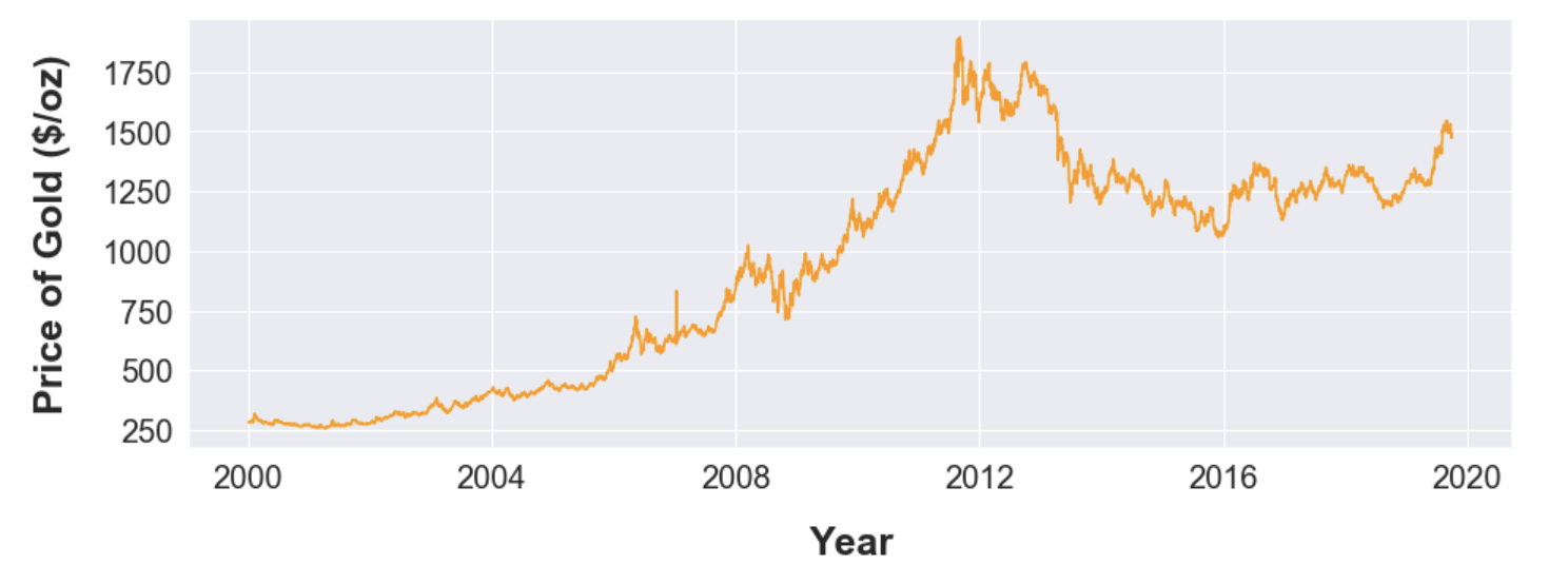
The dependent variable, price of gold, was collected from kitco.com website and is based on the London Gold Fix benchmark. This benchmark price of gold is set by a group of participating international banks twice every business day in London as the name indicates, and is used for pricing majority of gold derivatives and products throughout the world markets. The highest of the two rates set each day was used for this analysis. The gold prices used for this project are shown below:
The database was assembled from multiple soruces as lised below, and stitched together using dates as the merging attribute. Once the data were “stitched” together, US holidays were removed from the analysis. In addition, any missing or unreasonable data tagged during an Exploratory Data Analysis step was imputed using the prices from the previous day (forward filling).
Modeling
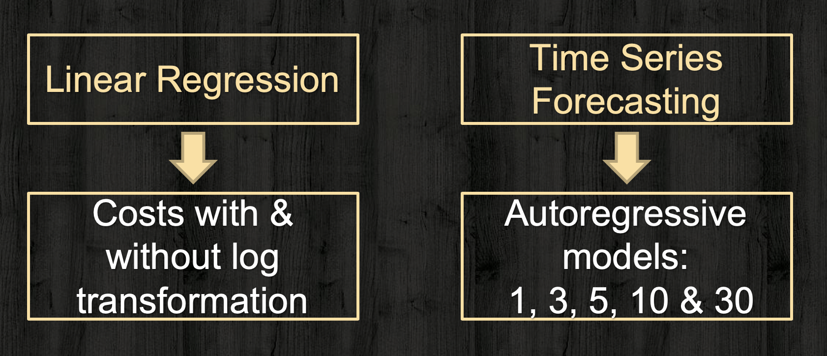
As part of the model builing exercise, linear regression and time series methods were used as shown below.
The model building process had gone through the following steps, where each step went through multiple iterations as needed:
- Use daily prices from 2000 to 2015 to train linear regression models. Dependent variables tested as part of this step include: next day’s price, next week’s price, next month’s price, and percentage change for next day’s price. These models were then tested using the daily prices for 2016 to 2018. The outcome of this step was to use next days price as the dependent variable and use only one-year for model testing instead of three years. It was noted during this step that the performance of the model deterioates as farther the testing data gets from the training data.
- Use daily prices from 2000 to 2015 to train linear regression models with costs log-transformed and scaled to center over zero. Test using the daily prices for the year 2016.
- Use daily prices from 2000 to 2015 to train univariate time series models using gold prices with and without log-transformation. Test using the daily prices for the year 2016.
For time series models, only autoregressive (AR) models were used. For two time series functional forms explored, with and without log-tranformed gold prices, the optimal order was determined to be 3 preceding days based on the Akaike Informational Criterion (AIC).
Model Evaluation
A critical step in evaluating the model performance for a time series vaiable like gold price is to compare the results against a naive solution. In case of a non-seasonal variable like gold price (as opposed to a seasonable variable like cotton prices or traffic volumes), the naive forecast is tomorrow’s gold price is same as today’s. Naive solution has limited utility as an investment strategy or decision making tool, but it makes a benchmark solution for model evalutation. For model building steps 1 to 3 mentioned in the previous section, the metric used in model selection and comparing agaist the naive solution is R-square value.
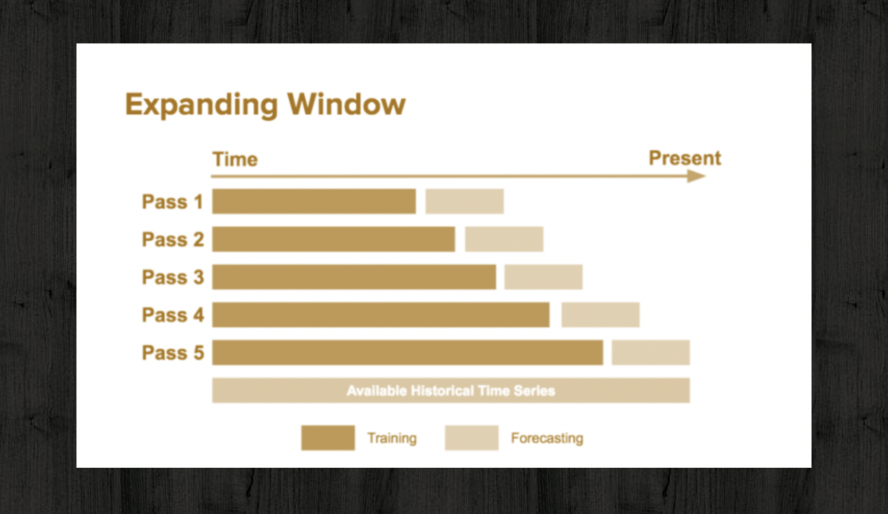
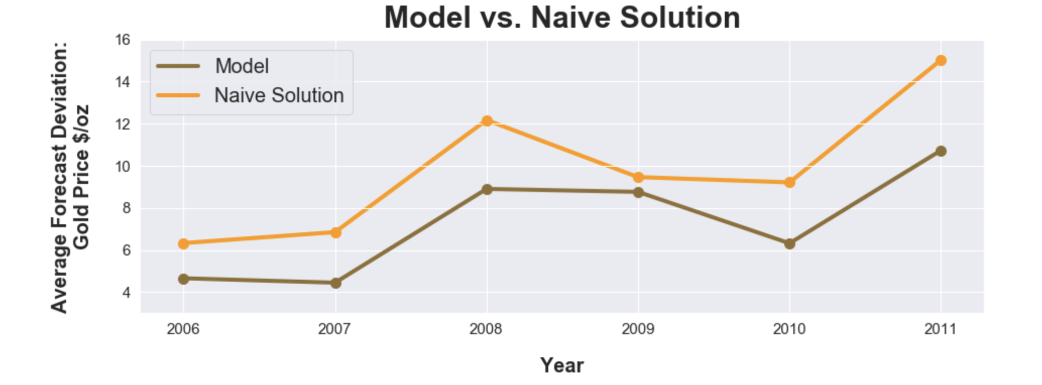
Once a model was selected, that functional form was used in performaning a chronological training/testing using an expanding window concept as shown below. Chronological training/testing was done for daily prices for every individual year from 2006 to 2018, using models that were trained with the data from the preceding years beginning with year 2000. For this chronological testing, Mean Absolute Error (MAE) was used for comparing against the naive solution.
Results
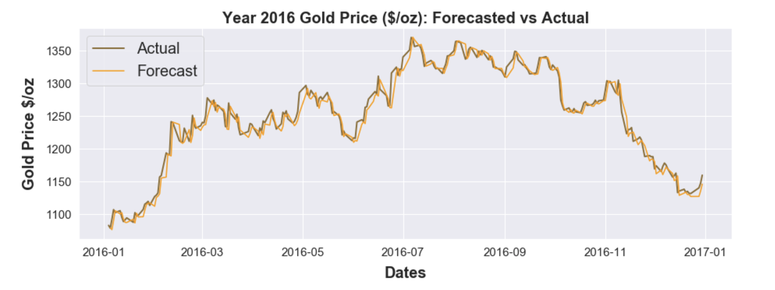
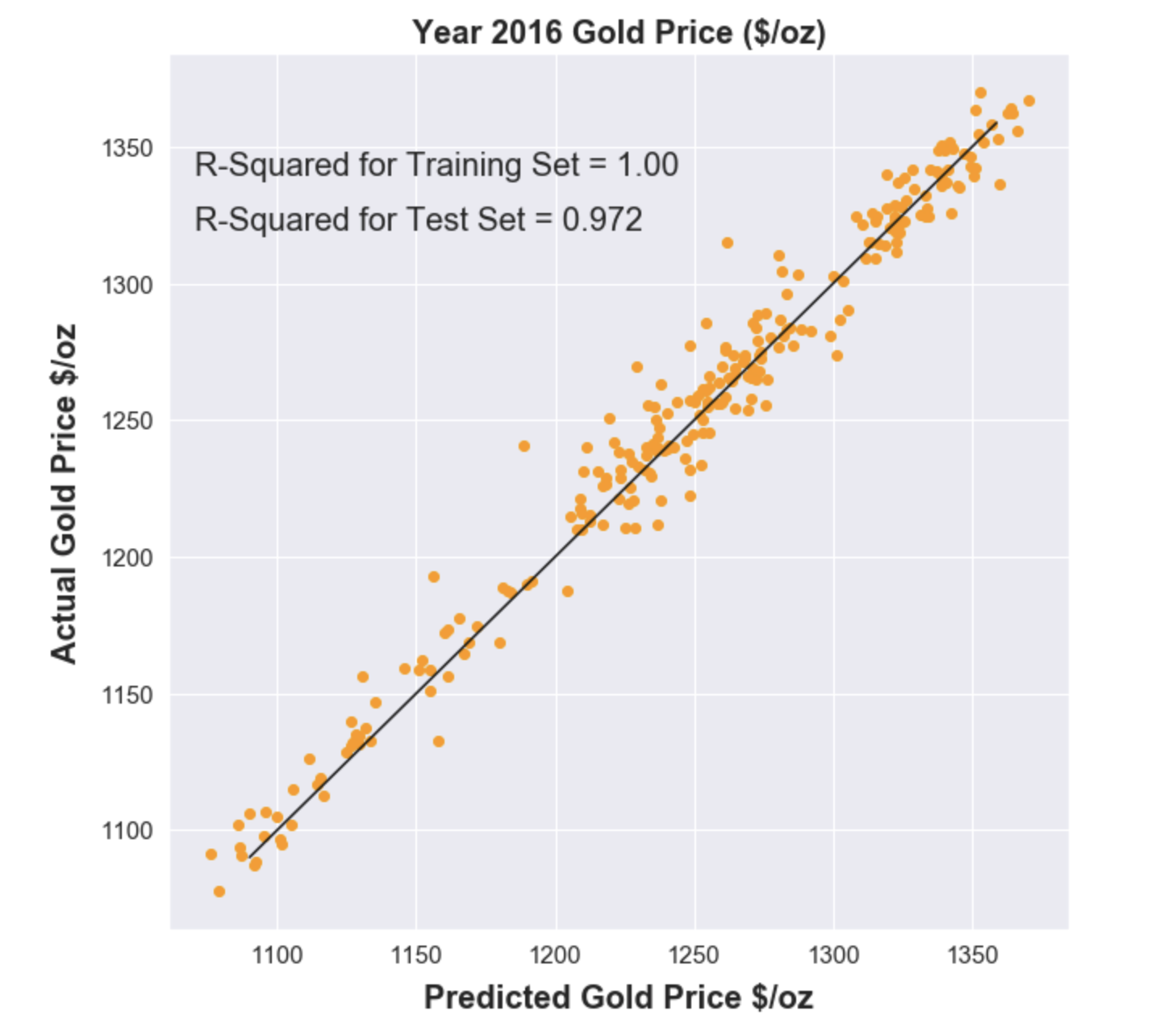
Test results for the year 2016 from the model building step for simple linear regression are presented below. This model was trainined using the daily gold prices from 2000 to 2015, and produced the best R-squared value compared against the naive forecast (0.9719 vs 0.9715). The model tracks pretty well with the actual 2016 gold prices, as demonstrated below:
A scatterplot of forecasted 2016 gold prices vs actual gold prices is shown below.
Chronological training/test evaluation performed using the linear regression models are presented below for the years 2006 to 2012. For every single year in this timeframe, the forecasts are closer to the actual than the naive forecasts. Average forecast deviation is measured using the mean absolute error (MAE).
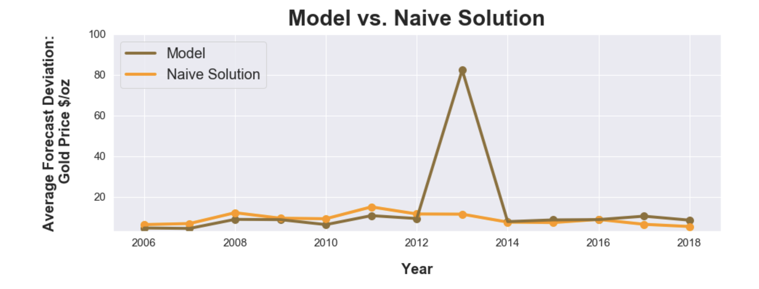
Chronological training/test results for 2006 to 2018 are shown below. Notice how the model failed to capture the shifting trends in the gold market occured in 2013.
What happened in 2013?
A huge swift in investments from precious metals to equites resulted in near 30% loss in gold prices in 2013 ending a 12-year bull market. This drop is primarily related to investors speculating US Federal Reserves cutting down their bond purchases removing any need to purchase gold as a hedge against US Dollar and inflation (WSJ Article).
The model estitmated using 2000 to 2012 training data was unable to fully capture the changing market conditions between equties, t-bills, US dollar, Federal Monetary policies, and the commodities markets.
Conclusions
The above historical analysis to model gold prices using linear regression and time series resulted in the following conclusions:
- For time series variavbles, always compare against a naive solution whether its possible to beat it or not.
- Check how far your model can hold and extend the trends. Not all models can completely generalize a highly complex system like stocks and commodity markets. Aim for a smaller timeframe and update frequently.
- Multiple models: have multiple models. Even if time series didn’t performe better than the naive forecasts, it would have captured the 2013 gold price drops better than the linear regression that did well against naive forecast.