Introduction
According to 2018 Used Car Market Report & Outlook published by Cox Automotive, 40 million used vehicles were sold in the US last year. This represents about 70% of the total vehicles sold. A good portion of these sales already use online resources along various stages of purchasing: searching, pre-qualifying, applying and finally buying. Popular websites for car buyers include AutoTrader.com, Kelly Blue Book, Cars.com, Carvana.com.
Cox Automotive’s report indicates that most market leaders and Silicon Valley startups speculate that car sales will shift completely to online retailing. This might be an extreme speculations, but these market leaders are interested in providing better user experience while buying a car online, and better recommender systems when a user searches for cars. Peer-to-peer sales platforms like Craigslist, Shift, eBay Motors etc are also interested in better fraud detection and monitoring of user postings.
A car image classification system can address these business issues:
- Ground-truthing of posted used car images on peer-to-peer sales platforms - are these images actually the cars they specify? Do multiple exterior pics represent the same car?
- Organizing web-page displays based on the user uploaded images
- Recommending alternative cars available in the inventory that have similar looks and price
In addition, a simple classification system of cars can help in identifying the fine-grained features important for 3D object detection for self-driving cars.
Approach
The approach used for this analysis has three stages: feature extraction stage, model building stage, and a model evaluation/error analysis stage.
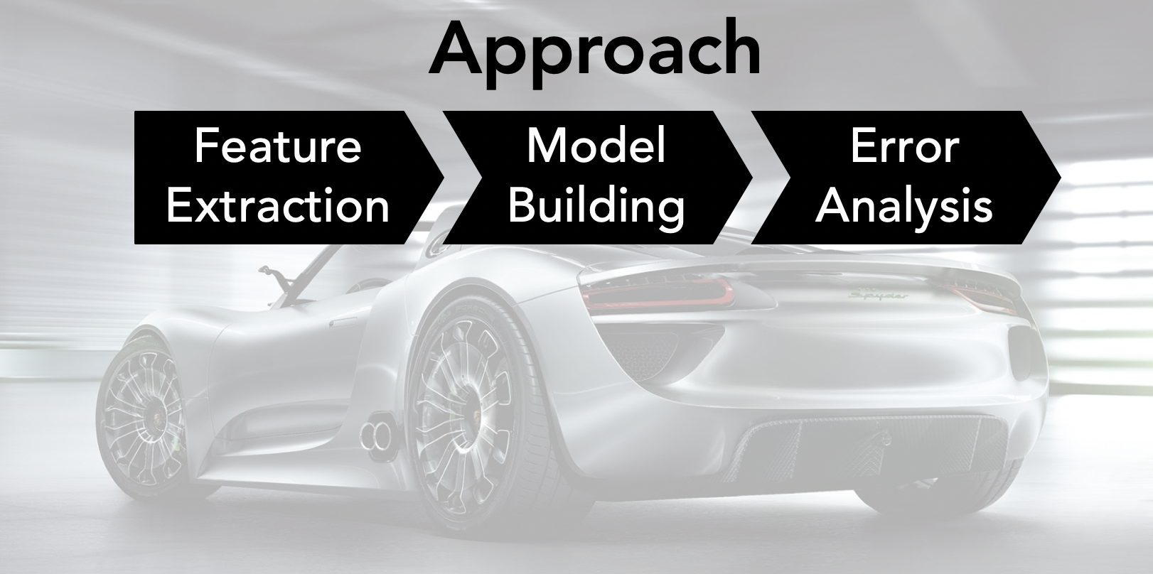 Figure 1: Approach Used for the Analysis
Stanford’s car image dataset was used for this analysis. This dataset consist of 16,185 total images (train set + test test) labeled with 196 classes based on the car’s Make/Model/Year. These images come in various sizes and resolutions. For this analysis, the 196 image labels in the dataset were consolidated to five vehicle types as shown in the figure below. Although these represent somewhat ‘crude’ consolidation of vehicle types, they proved to be more manageable, and adequate for the image classification task.
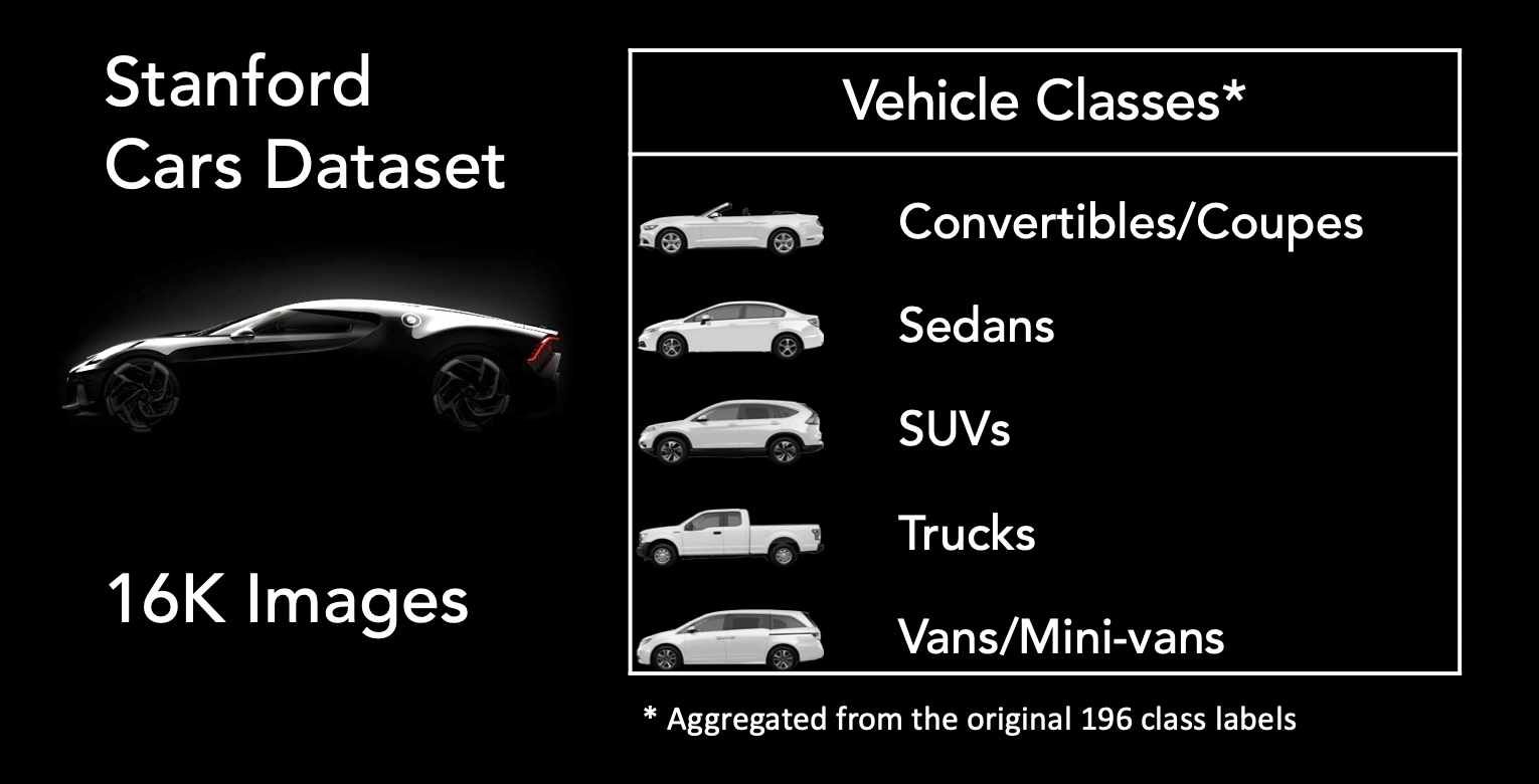 Figure 2: Vehicle Classes Used in the Analysis
Feature Extraction
Features for each of the car image were extracted from Deep Learning Convolutional Neural Networks (CNN) with weights pretrained on ImageNet dataset. The creators of these CNNs provide these weights freely, and modeling platform Keras provided a one stop access to these network architectures and weights. Overall, five CNNs, as shown in the figure below, were used in extracting the features and were separately used for classification task to compare which deep learning architecture performed the best. The features extracted were from the first fully connected hidden layer above the final softmax layer.
| CNN Model | Input Image Size Requirement | Number of Features Extracted1 |
|---|---|---|
| VGG 16 | 224 x 224 | 4,096 |
| VGG 19 | 224 x 224 | 4,096 |
| ResNet50V2 | 224 x 224 | 2,048 |
| InceptionV3 | 299 x 299 | 2,048 |
| MobileNetV2 | 224 x 224 | 1,280 |
1Features were extracted from the fully connected hidden layer above the final softmax layer. Figure 3: Vehicle Classes Used in the Analysis
Model Building
The first step performed in the model building stage was reducing the dimensionality of the extracted features. This step helped in bringing the dimensions of the features to a manageable number and increases the speed of iterative model building step. Dimensionality reduction was performed using Principal Component Analysis (PCA), and a systematic search resulted in using a reduced dimension of 500 features that captured about 85-90% of the variance in the features across five CNNs.
The original dataset has roughly 50-50% train-test split. For this analysis, these tests were combined together and a train-test split of 80-20% was used. Train-test sets were established such that the class distribution is maintained.
A number of classification methods were employed in this stage of the process. These include: Logistic Regression, Random Forests, SVMs with polynomial kernels, XGBoost, and a shallow neural network (Multi-layer Perceptron classifier from sklearn).
The dataset after consolidating to five classes has a class imbalance with Vans representing about 6% of the data and on the other extreme Convertible/Coupes and Sedans each representing about 32% of the data. To address this class imbalance the above classification methods were iterated with oversampling techniques: random oversampling, and Synthetic Minority Oversampling TEchnique (SMOTE).
In addition, a stacked classifier was tested to see if combining the results from the best Logistic Regression and Random Forest models will yield better results than either of them could individually.
Model Results and Error Analysis
For comparing the model performance, multiple metrics were considered. But after few iterations, accuracy was noted to be a sufficient metric to assess the model performance. Selecting any other metric (say F1 Score) would have resulted in arriving at similar conclusions. A detailed error analysis was performed by examining the misclassified images and exploring any similarities in these mis-classifications.
Results
The results of the best performing models are presented in the following figure. As seen below, the model using features extracted from InceptionV3 performed best in general, with Logistic Regression resulting in slightly better accuracy than Random Forest. Model using InceptionV3 features, Logistic Regression with L2 regularization, and random oversampling technique was selected as the Preferred Model for this analysis.
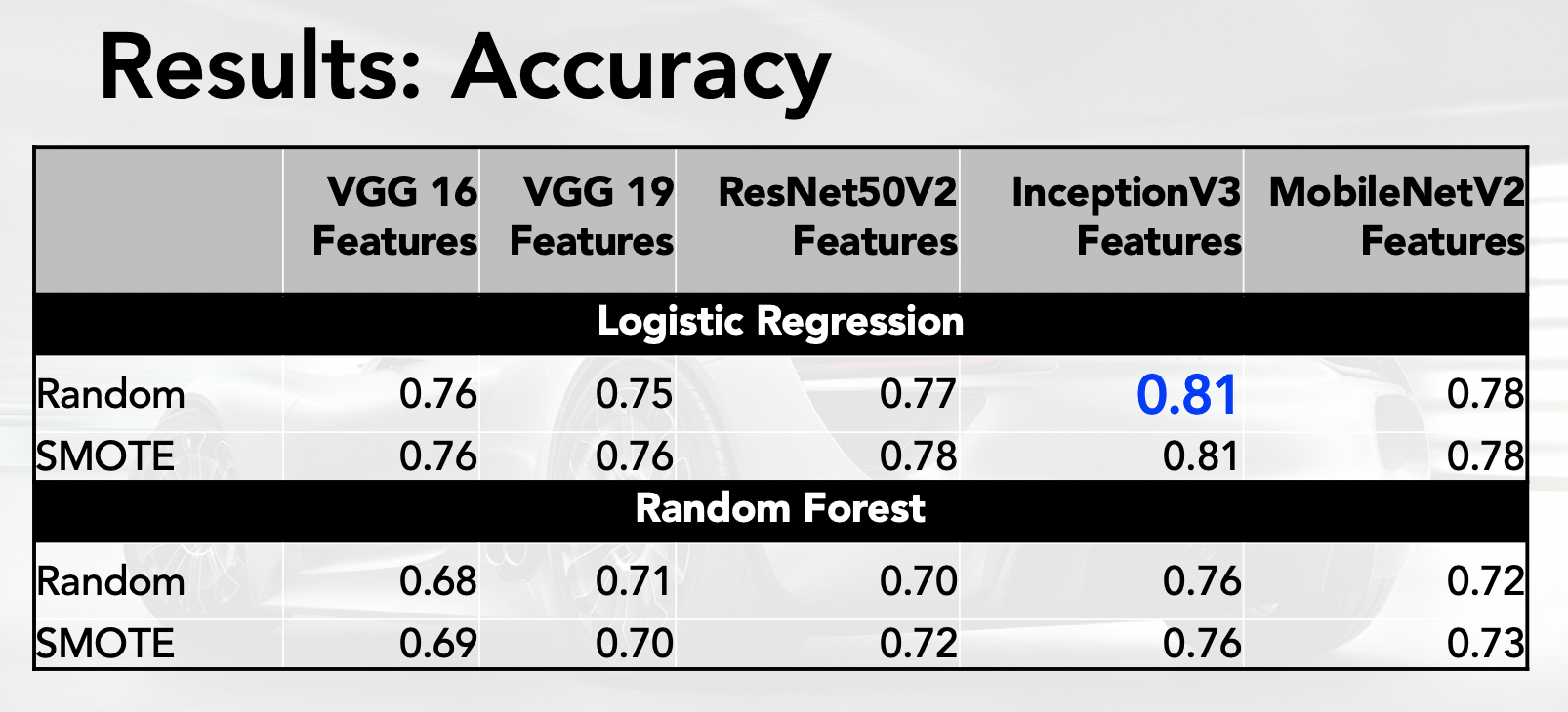 Figure 4: Comparison of Model Accuracy for Select Runs
Confusion matrix for the preferred model is presented in the figure below:
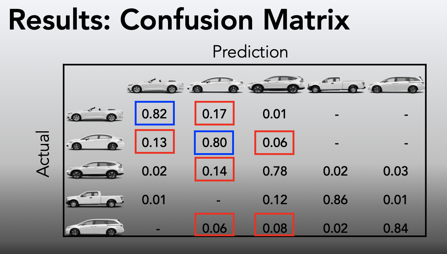 Figure 5: Confusion Matrix for the Preferred Model(InceptionV3 Features + Logistic Regression)
In addition to tracking the model accuracy, a detailed error analysis was performed to assess where the model is performing poorly. This error analysis was critical in performing a quality check (QC check) on the class labeling, identifying model “blind spots” and future improvements.
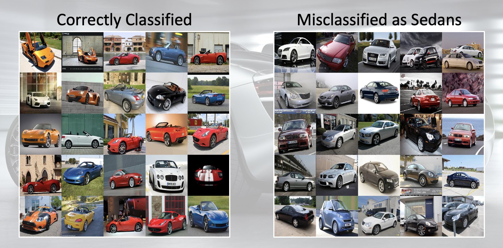 Figure 6: Error Analysis of Convertibles/Coupes for for Preferred Model
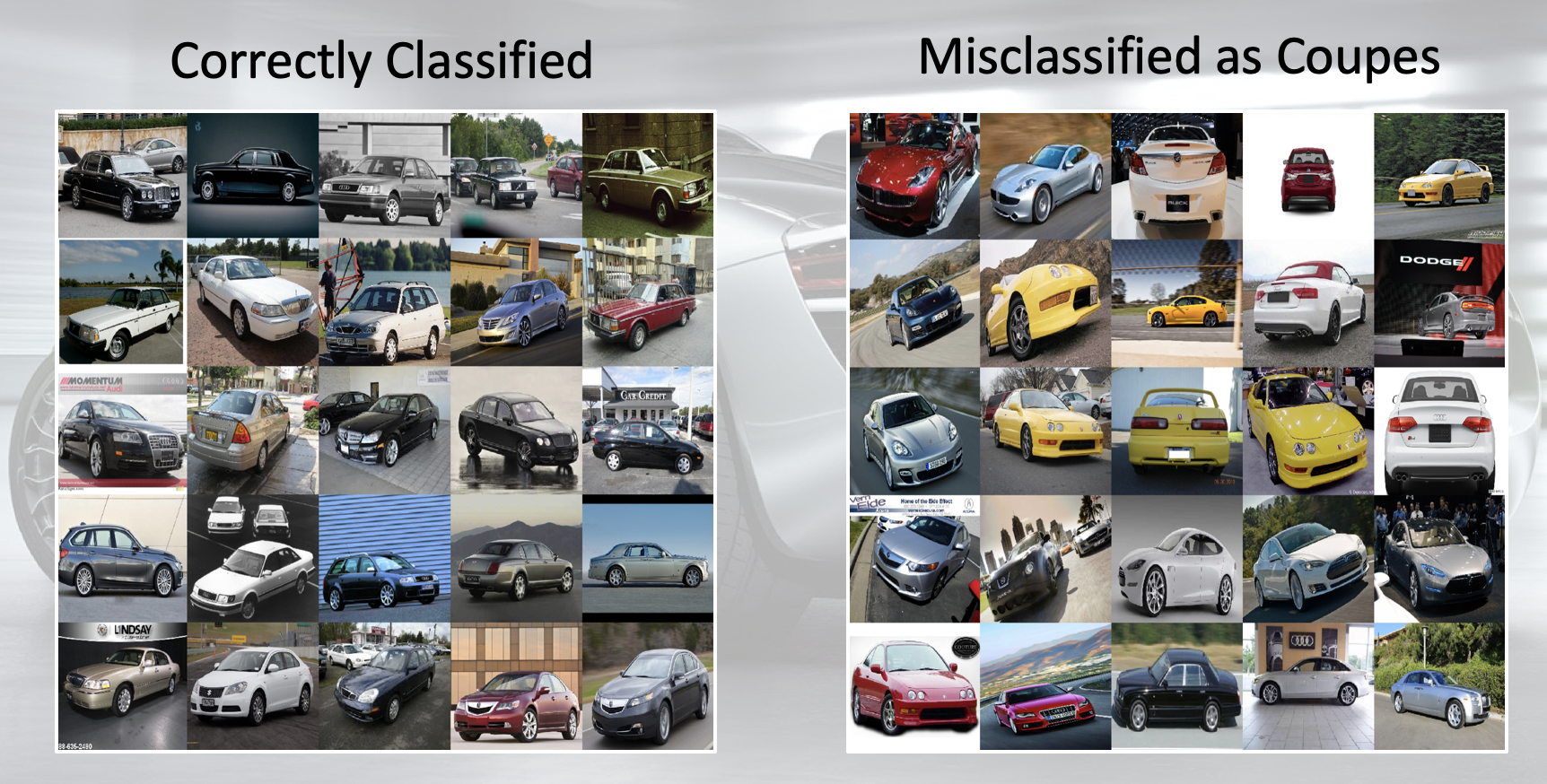 Figure 7: Error Analysis of Sedans for the Preferred Model
As seen in figures 6 & 7 above, the model seem to pick up colors as classification feature. Convertibles/Coupes correctly identified are rich in color, while those misclassified as Sedans are less colorful. Likewise, as seen in figure 7, Sedans that are misclassified as Convertibles/Coupes are more colorful than the Sedans that are correctly classified. This is an encouraging result in most cases as this will pick up colors specific to certain car Make/Model but the weight placed on color is higher than the weight placed on features that represent shape and size.
Conclusions
The primary conclusions from the above image classification analysis are:
- Prototyping a classification model using pretrained CNN features is quite effective and easier than fully building a deep neural network from scratch.
- Error analysis is quite useful, and provides insights on how models can be employed.